Supervised Image Classification

This week we worked on Lab 10 which allowed us to create spectral signatures and AOI features. We were able to produce classified images from satellite data given.  We were able to recognize and eliminate spectral confusion between spectral signatures. The map shown is a Land Use map of Germantown Maryland. The different color indicate different land uses, we had to create the SIG file from an Image file in order to be able to classify the different land uses.

Unsupervised Classification Lab9

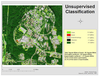
This week we worked in ERDAS to label features in an image under categories. We were able to take the image of the UWF campus and classify it.
 The map below is a map that shows the UWF campus. The colors in the legend signify the different land features of the image.

Thermal & Multispectral Analysis, Lab8 4035

This week we got to toy with Composite bands in Arcmap, and Layers Stacks in ERDAS. In my map I chose to show the fires in Florida. I chose this image for the fires would show better thermally in comparison to the land, for me to get the image to where I wanted it, I stretched the image and chose band 6, then I color ramped the image from red to blue, then I adjusted the DN value in the Histograms, to 14 and 40. The blue color in the image shows the cooler objects, and the yellow and red images are the objects that are thermally hotter.

Spatial Enhancement, 4035 Photographic interpretation and Remote Sensing

   This week we focused on Multispectral Analysis. Multispectral Analysis dealt with image enhancing ,adjusting breakpoints and LUT Histogram, we learned how to select different layers in the panchromatic tab to adjust our image so we can enhance the image to show different features.
   In the first map we had to chose an area where in Layer 4 it had the spike range of 12 and 18. I noticed that in Layer 4 the area that had the change was the water. So I chose an image of the water for Feature 1.

For my second map they lab wanted us to identify a feature that both represented a small spike value  in Layer 1-4, but a large spike pixel value in Layers 5 and 6. In the map I chose to show the mountain range for in Layers 1-4 the features were bright, and in Layers 5-6 the features were dark.

Map three shows the image of an area of water that in Layer 1-3 was brighter than normal, but in Layer 4 become somewhat brighter, and in Layers 5-6 remain unchanged. In the map I chose to show an image of Lake Tapps for my 3rd feature.

Spatial Enhancements,

This week we were able to familiarize ourselves with Glovis at the USGS website. We were able to download Landsat images from USGS's archive. We also got to convert TIFFs and  filter them through different filters. In Arcmap we were able tp filter imaged using Focal Statistical Analysts. In ERDAS we were able to convert Striping image into a visible map image.

In the image above it shows the outcome of a striping image once it has been converted into a visible image. After the image was converted it was enhanced in Arcmap using the focal spatial analysts.

Intro to ERDAS Image and Digital Data 1

This weeks lab we learned a few calculations such as Maxwell's wave theory, and Planck's relation,both which are needed when calculating EMRs. We also got to learn and use a new system called ERDAS. ERDAS is a beginning processing step for making Arc maps.
   The Arc map displayed was made from data created on  ERDAS. The picture was then used to create this map in Arc map. The map represented different terrain types, and the square acres of that terrain,within the  Olympic Mountains, located in Seattle, Washington.

Truthing Lab4

I started the Truthing lab with my previous lab3 arcmap. In this lab I randomly placed 30 points on my existing LULC arcmap. The lab allowed us to compare the over all land code to the actual land usage of the points. The points on the map signifies if the land use and land codes on the map match the land usage of the actual point.